eMMA INSPECTOR
2019-03-14 - Powerful interactive analysis of large datasets at your fingertips
| Name | Usage | Duration |
|---|---|---|
| privacylayer | Status Agreement Cookie hint | 1 year |
| Name | Usage | Duration |
|---|---|---|
| _ga | Google Analytics | 2 years |
| _gid | Google Analytics | 1 day |
| _gat | Google Analytics | 1 minute |
| _gali | Google Analytics | 30 seconds |

05 May 2014: Michael Radeck
In case you measure parts with a three-dimensional coordinate measuring machine, each measured value is defined by its x-position, y-position and z-position. Characteristics whose location in space is specified by three coordinates are referred to as “position characteristics”. Engineering drawings often specify the tolerance for each axis separately (tolerance = permissible deviation from the nominal value). We refer to this type of tolerancing as one-dimensional tolerancing. However, the one-dimensional tolerancing is the wrong approach for multidimensional characteristics. First, we want to confirm this statement based on a transparent example including two dimensions. The distance from the nominal value = tolerance center to the upper specification limit is equal to the distance from the nominal value to the lower specification limit in the first dimension. However, in case the characteristic varies in two dimensions, the permissible distances from the nominal value to the respective specification limit suddenly differ. The nominal position is exactly in the middle of the tolerance square (see x/y-plot). If you measure the distance from the middle of the square to one of the corners of the tolerance square, you will find out that the distance is longer than the distance from the nominal value to the middle of one of the sides. As a result, the permissible deviations will differ considerably depending on the respective direction if you actually use the tolerance square. However, there is a solution to this problem. You have to use the tolerance circle whose radius complies with the range from the nominal value to the upper specification limit of the one-dimensional approach. The radius ensures that the maximum permissible distance from the nominal value is equal in all directions.
The nominal position of a borehole is defined by xnom = 100 mm and ynom = 75 mm. The specification limits for the x-coordinate are USLx = 100.05 mm and LSLx = 99.95 mm whereas the specification limits for the y-coordinate are USLy = 75.05 mm and LSLy = 74.95 mm. Now we measure the borehole position of 50 parts. The following figure shows the one-dimensional measured values of each axis separately (in the value chart) and their two-dimensional dispersion (in the x/y-plot). Measured values taken from a two-dimensional normally distributed population create a random dispersion ellipse.
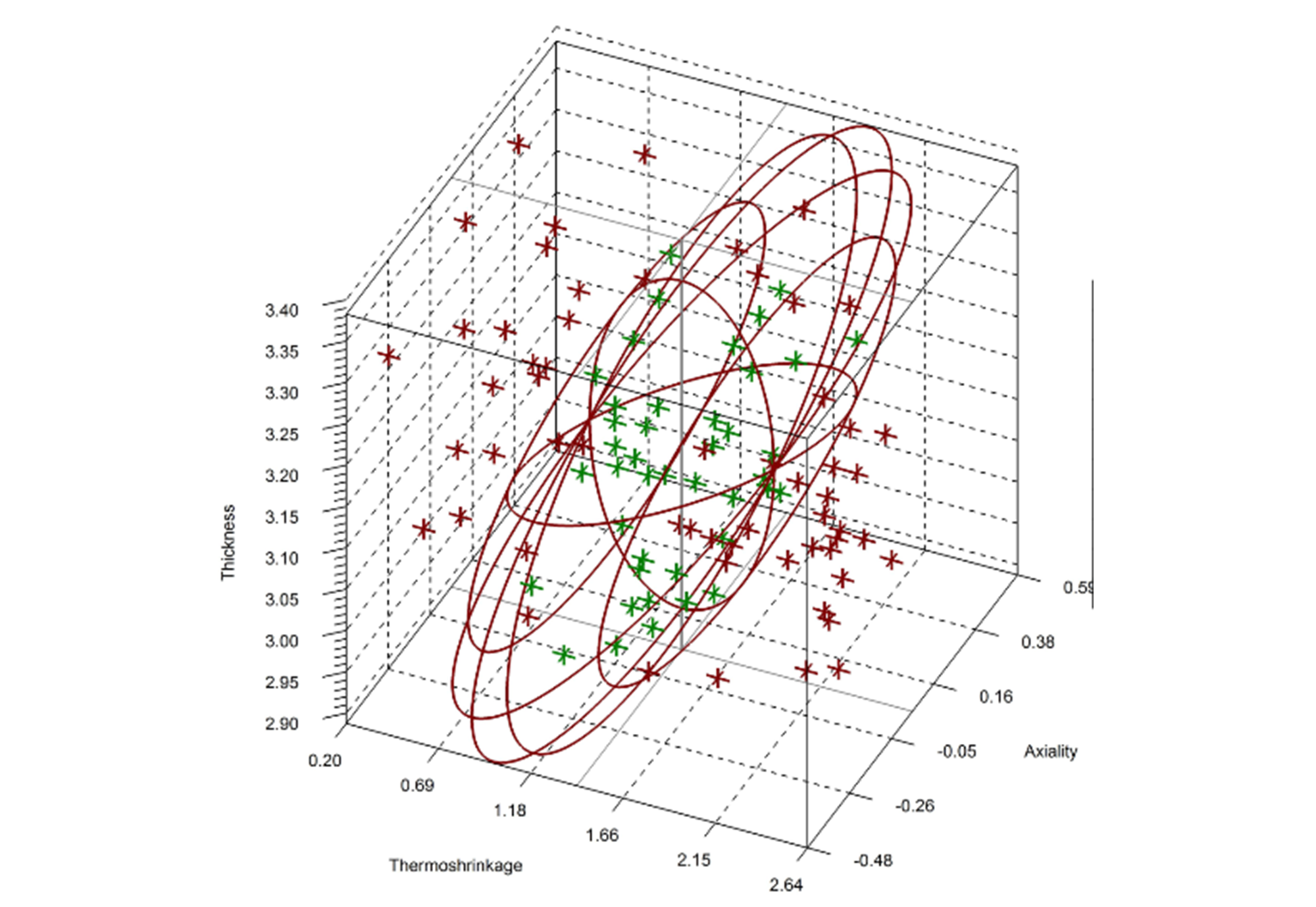
The behavior in the first dimension can be translated into three dimensions. In this case, the tolerance is just a tolerance circle or, in general, a tolerance ellipsoid. When the measured values are taken from a normally distributed population, the values create a random dispersion ellipsoid whose shape resembles an American football...